This illustrative project involves the entire tree matrix for the intermediate steps to implement the Binomial Options Pricing Model.

The Binomial Model is a lattice-based approach that uses a discrete-time model of the varying price over time of the underlying financial instrument. First proposed by Cox, Ross, and Rubenstein in 19791. Binomial option pricing is a simple but powerful technique that can be used to solve many complex option-pricing problems.

Binomial Tree Approximation

Theoretically, the Black Scholes formula, the continuous-time pricing formula, can be approximated by the step increments of binomial tree models. Binomial trees are a discrete pricing model in which we can derive the option price by

where \(Z_{n}=X_{1}+...+X_{n}\) is the corresponding random walk.

To accomplish the binomial tree approximation, we can let the steps (n) in the formula go to infinity. By the Central Limit Theorem, we know \(Z_{n}\) is very close to a normal distribution so that \(\mu(Z_{n})=n\mu(X_{1})\) and \(\sigma(Z_{n})=\sqrt n\sigma(X_{1})\). Applying that to the continuous-time stock price model, we have \(\frac{Z_{n}lnu-E(Znlnu)}{\sigma(Z_{n}lnu)}\sim N(0,1)\).

By further induction, we can show that the option price

where \(W_{T} \sim (0,T)\). Applying the pricing formula to European call, we can then derive the formula in the last section.

Note: this is only one way of deriving Black Scholes formula, which arguably is not the fastest method. But it’s the first one that I got exposure to and is very intuitive.

Numerical Calculation

To conduct the numerical approximation of the binomial tree model to the Black Scholes, I chose to implement the numerical process in R - the statistical programming language that allowed me to code out specific steps. For convenience, I set up a series of functions that roll out the necessary steps in calculating the price of the European call at time 0. First, I created a function that returns risk-neutral probability (function rn_prob(r,deltaT,sigma)) for use in future steps. In this function, up (\(u = e^{\sigma\sqrt\Delta_{t}}\)) and down (\(d = e^{-\sigma\sqrt\Delta_{t}}\)) factors were set up using the formula under the Cox-Rox-Rubinson condition.$\vspace{0.2cm}$\

#first set up a function that rolls about risk neutral probability
rn_prob = function(r, deltaT, sigma) {
  #up factor
  u = exp(sigma*sqrt(deltaT))
  #down factor
  d = exp(-sigma*sqrt(deltaT))
  #R
  R = exp(r*deltaT)
  return((R - d)/(u-d))
}

#then construct the matrix that sets up the binomial tree 
stock_tree = function(S, sigma, deltaT, N) {
  treem = matrix(0, nrow=N+1, ncol=N+1)
  #up factor
  u = exp(sigma*sqrt(deltaT))
  #down factor
  d = exp(-sigma*sqrt(deltaT))
  
  for (i in 1:(N+1)) {
    for (j in 1:i) {
      treem[i,j] = S * u^(j-1) * d^((i-1)-(j-1))
    }
  }
  return(treem)
}

Similar to what we do for manual calculation, I hoped to construct a tree through the program and realized that a matrix (stock_tree(S, sigma, deltaT, N)) can help achieve the goal. There are N+1 steps in the multi-step binomial tree model so I set up a $(N+1)\times(N+1)$ matrix and on the ith row and jth column, the stock price is $S\times u^{j-1} \times d^{(i-1)-(j-1)}$.

Next, another function (option_value(tree, sigma, deltaT, r, k)) builds the option tree upon the stock tree. While the tree model in the previous function sets up the stock prices, the function reads in the tree and other parameters and calculates the actual value on each node. Since we are doing calculation on European call, the call formula \((S-K,0)^{+}\) is used. Then the payoff on each node is \(\frac{(1-p^{*})*optiontree[i+1,j]+p^{*}*optiontree[i+1,j+1]}{e^{r\Delta T}}\).

#since this is a call here we are only considering the situation of call here
option_value = function(stock_tree, sigma, deltaT, r, k) {
  pstar = rn_prob(r, deltaT, sigma)
  option_tree = matrix(0, nrow=nrow(stock_tree), ncol=ncol(stock_tree))
  option_tree[nrow(option_tree),] = pmax(stock_tree[nrow(stock_tree),] - k, 0)
  for (i in (nrow(stock_tree)-1):1) {
    for(j in 1:i) {
      option_tree[i, j] = ((1-pstar)*option_tree[i+1,j] +pstar*option_tree[i+1,j+1])/exp(r*deltaT)
    }
  }
  return(option_tree)
}

Finally, an ultimate function (option_price(sigma, T, r, k, S, N)) directly calls on the previous trees. This function takes the following parameters by order: volatility, expiration time, annual interest rate, strike price, stock price and steps. The option tree is based off the stock tree and I can retrieve the desired option price from (1,1) of the option tree matrix.

option_price= function(sigma, T, r, k, S, N) {
  stock = stock_tree(S=S, sigma=sigma, deltaT=T/N, N=N)
  option = option_value(stock, sigma=sigma, deltaT=T/N, r=r, k=k)
  return(list(option=option,price=option[1,1]))
}

Using the option_price() function, we can manipulate the parameters to compare the outcome. In this project, my goal is to explore the convergence of call price when the steps in binomial tree increase thus I hope to change the steps (N) and to compare the resulting call price. Regarding the scaled parameters, though not specified, since \(\Delta T = \frac{T}{N}\), I noted that the volatility is scaled by \(\sqrt{\frac{T}{N}}\).

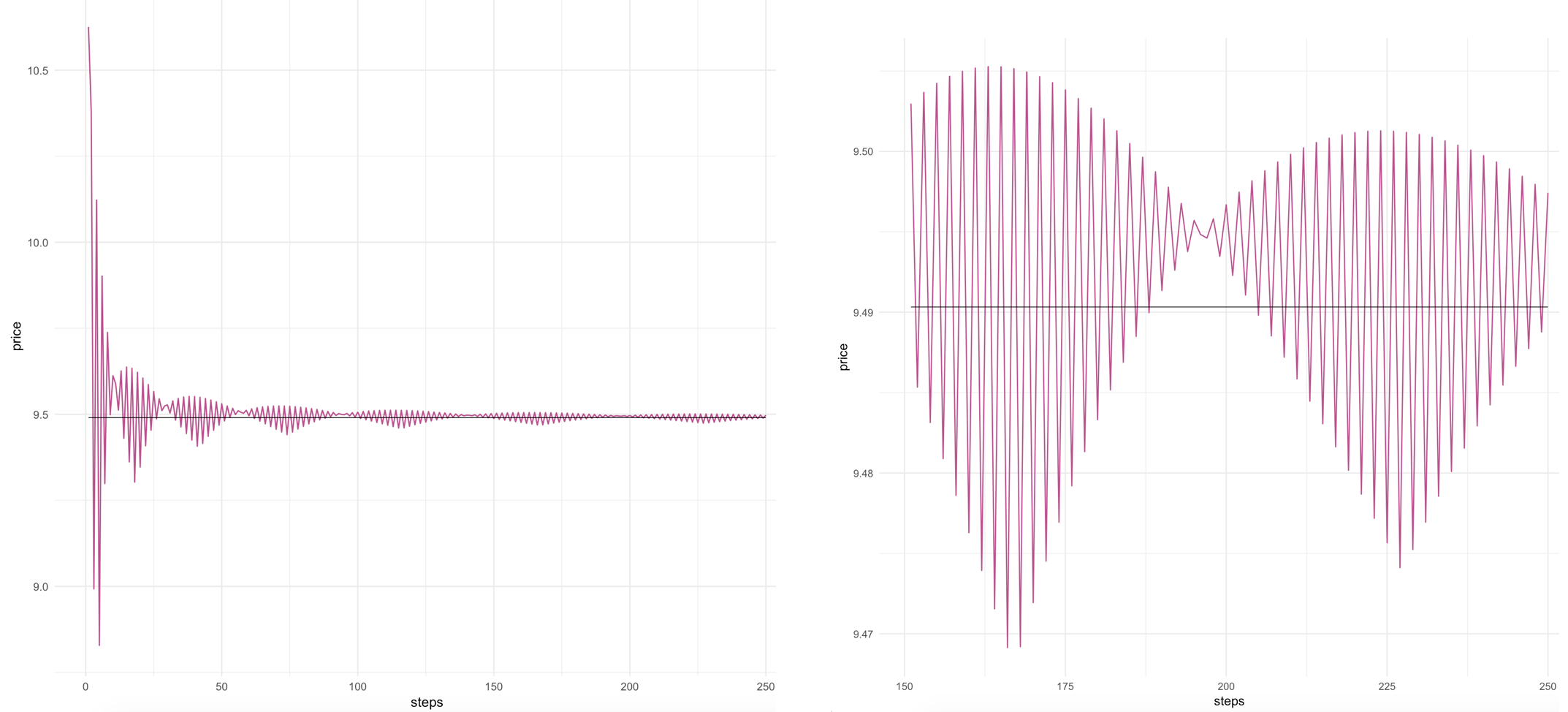
For the approximation process, I started from 10-step binomial tree and the resulting call price is relatively far away from our target price ($9.49). Then I increased the steps to 50, 100, 150, 200 and 250. When there were 50 and 100 steps, the resulting prices were $9.5307 and $9.5068 respectively. As the steps gradually increment, the absolute differences between the price from Black Scholes formula and my calculted price decreased to 0.003 (which is less than 1 cent) when I incremented to 150 steps. There were fluctuations in the prices but the differences became more and more minimal. I realized that picking out specific steps only captures crude snippets of the convergence so I decided to initialize a “for” loop and repeated the calculation for every single step (see code). Through the loop, I looked for the steps where I had the closest approximation and also tried to graph the convergence out.

library(ggplot2)
library(tidyverse)

steps <- 1:250
price_change <- data_frame(steps,price)
price_change <- price_change %>% add_column(bs_price=9.490328)
price_change %>% 
  ggplot(aes(x=steps))+
  geom_line(aes(y=price),size=0.5,color='#bc5090')+
  geom_line(aes(y=bs_price),size=0.3,color='black')+
  theme_minimal()
#if we zoom in
price_change %>% 
  filter(steps>150) %>% 
  ggplot(aes(x=steps,y=price))+
  geom_line(size=0.5,color='#bc5090')+
  geom_line(aes(y=bs_price),size=0.3,color='black')+
  theme_minimal()

*Note: this gets slower as period increases since this is at \(O(N^{2})\). Some research leads me to a parallel implementation using the library parallel if we want to do something more complicated in the future.

Black Scholes Formula Computation

For comparison, let’s use Black Scholes formula.

The Black Scholes formula is used to calculate the theoretical value of European options using current stock prices, the option’s strike price, expected interest rates, time to expiration and expected volatility. The call price is

where \(d_{1} = \frac {ln (S/K) + (r+\sigma^2/2)t}{\sigma\sqrt{t}}\) and \(d_{2} = d_{1} - \sigma\sqrt{t}\).

The formula is divided into two parts: the first part multiplies the current price by the change in the call premium relative to the change in the underlying price. It represents the expected benefit of purchasing the underlying option. The second part gives the present value of paying the strike price on expiration and the call price is calculated by the difference of the two parts.\

In this project, Strik price = $120, Expiration time = 1 yr, annual interestrate=0.07, volitility = 0.3, current price = $104.4. By plugging the parameters into the Black Scholes formula, I figured that the theoretical value of this call option is $9.490328.

Just out of curiosty, I tried to figure out which step produced the call price closest to the desired one.

dif={}
price={}
abs_dif={}
for (i in (1:250)) {
  price[i]=option_price(0.3, 1, 0.07, 120, 104.4, i)
  abs_dif[i]=abs(option_price(0.3, 1, 0.07, 120, 104.4, i)-9.490328)
  dif[i]= option_price(0.3, 1, 0.07, 120, 104.4, i)-9.490328
}
N=which.min(abs_dif)

When there are 188 steps (N=188), the multi-step binomial model achieved the closest approximation with the price of 9.489976. Let’s have a look at a small snippet of the binomial tree at 188 steps.

From graph (zoomed in on the right) and the calculation, I observe that
1) the variation of the option price has been decreasing when steps increase, i.e. the call price by binomial tree approximation shows a conspicuous pattern of convergence. After we reach more than 150 steps, the difference is kept under 2 cents.
2) steps of odd numbers tend to underestimate the call price while even numbers overestimate,
3) when there are 188 steps (N=188), the multi-step binomial model achieved the closest approximation with the price of $9.489976 with absolute difference less than 0.1 cent.