Comparative High Frequency Trading Analysis on the Microstructure Behaviors of Three Common Stock

Research Goal

In this research, we hope to perform a comparative high-frequency trading analysis on the mi- crostructure behaviors of three common stocks - BAC, GOOG, TSLA - using various feature data inspired by Microstructure in the Machine Age by Easley et al. Specifically, our research aims to

• Compare the underlying microstructure behaviors among the three popular and liquid stocks
• Extract an one-minute option-based trading strategy through comparing the predictive performance of machine learning models on bid-ask spread, estimated volatility and minute return

Data

We leverage our data analysis on the advantage of KDB database in its comprehensive trades and quotes offering of the NYSE trade-and-quote (TAQ) data, by which we establish our data engineering procedure using its Level 1 data. While the nbbo table lists the national best bid and offer across all exchanges, we mainly construct our features with the trades table for run-time consideration (with one exception of the imbalance metric).

Stock Selection

We choose BAC, TSLA, GOOG to perform analysis and compare the predicting power of our model among the three securities. The three equity securities are chosen for comparison because they are a good representation of common, popular and liquid stocks in the U.S. stock market, yet they not only cover relatively different industries, but also might entail distinct trading behaviors from investors.

Feature Construction

This section specifies our formulation on feature construction. Our dataset is limited to the three selected symbols (BAC, TSLA, GOOG) from February 4, 2020 to February 25, 2020. Only intraday data during trading time 09:30AM to 04:00PM of each date is included and we select rows that have a null condition code. Referring to Easley et al. (2019) and materials in class, we construct features as follows.

Bid-Ask Spread

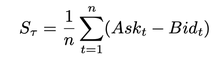
Since we construct the feature by each minute, Bid-Ask spread is computed by the average of (Ask - Bid) within that minute:

In Microstructure in the Machine Age, Corwin-Schultz high-low estimator is used as a proxy for bid-ask spread. We have decided to not proceed with it in our analysis because it yields a lot of negative values for the stocks we pick. As pointed out by Tremacoldi-Rossi and Irwin(2019), this high-low estimator misbehaves for the liquid assets with small spread.

Roll Spread

Richard Roll (1984) proposed an Implicit measure to estimate the effective Bid-Ask spread in an efficient market. The measure is classified by Easley et al. (2019) as the first generation measure. The implicit spread is given by,

Imbalance

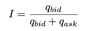The imbalance statistic shows how much bid and ask volume is on each side. If bid size is much larger than the ask size, we may predict that the stock price will more likely go up.

Amihud Illiquidity

We compute this illiquidity measure of each minute with a lookback window W = 5 mins. By computing average absolute return divided by dollar volume over a period of time, we can measure the illiquidity of a particular stock. For instance, if the stock moves a lot with high return but the dollar volume is not high, this will be an illiquid stock.

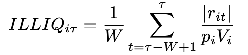
• rik is the return for stock i on minute k
• pik is the stock price for stock i on minute k
• Vik is the trading volume associated with stock price. pikVik is the dollar volume

Kyle’s Lambda

Kyle’s Lambda is a widely-recognized measure of market impact cost from the literature work by Kyle (1985). The measure can be interpreted as “the cost of demanding a certain amount of liquidity over a given time period.” There are various ways to estimate Kyle’s Lambda. For implementation efficiency, we follow the formula according to Easley et al. (2019) as follows.

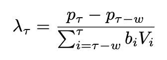
where b = sign[pi − pi−1], w = lookbackhorizon, V = size, p = price

The lookback horizon (w) is set at 5 minutes throughout.

Volume Synchronized PIN (VPIN)

The volume-synchronized probability of informed trading, proposed by Easley et al (2011), is classified as one of the third-generation models. It has its unique high-frequency advantage over the probability of informed trading (PIN) as PIN only offers daily estimations. VPIN, computed by ratio of order imbalance, is hereby estimated as below.

where OI=order imbalance,VBS=volume bin size, α=probability of information events occurs, μ=rate at Informed traders enter the market, ε=combined sell and buy rates

VPIN by its nature is using volume bars and our analysis focuses on the research on a minute-based trading strategy, a VPIN-missing minute is forward filled by the most recent value as a solution.

Estimated Volatility

To estimate the intraday volatility, we first generate a table with the open, high, low and close values from each minute of the trading day. Our next step is to apply the simplified Garman-Klass volatility measure (without averaging over observations) to estimate variance (volatility squared). The formula is displayed below.

$\sigma^2=\frac{1}{2}\left(\ln(\frac{h}{l})\right)^2-(2 \ln(2)-1)\left(\ln(\frac{c}{o})\right)^2$

Lastly, we use the mavg function to compute a moving average over a window of 5 minutes, annualize the numbers with 6.5 hours in a trading day and 252 trading days per year and convert the variance numbers to volatility.

Additional forecasting features include volume (size), minute return, minute high-low ratio.

Machine Learning Algorithms

With the microstructure feature set constructed, we apply the machine learning models to examine the predictive power of such explanatory variables. To start our machine learning pipeline, we frame our research problem into intraday next-period predictions, i.e. using features at time t to predict a selected measure at t+1. In our case, it is specified to be the next-minute prediction.

Since we hope to extract as much applicable information related to a plausible trading strategy as possible from the modeling results, we propose three candidate responses - bid-ask spread, estimated volatility and minute return. In addition, in order to ensure intraday “continuity,” we hope to circumvent inter-day confusions where features of the last entry of one day are used to predict the first entry of the next day. To remove such abnormal behaviors, we drop the corresponding rows in the data preprocessing process.

Machine Learning Framework

We apply LASSO Regression and Random Foreston the dataset. The first row of each date is dropped to rule out overnight fluctuation.

The LASSO Regression is a classic machine learning tool for prediction. By seeing the sparsity pattern, we can explore which variables are being used for prediction, which is essential for us to interpret our features.

We choose to implement Random Forest as it is one of the best all-around tools for prediction. Random Forest automatically performs variable selection and transformations, making them scale well with dimension. Important interactions are also automatically detected by Random Forest and can be examined by the partial dependence plot, avoiding the need to recognize and specify explicitly.

In order to assess the performance of LASSO and Random Forest, we define the benchmark model as $y_{t+1}=y_t$, which we use the value of the response y at the current time period as the prediction for the next period.

Error Metric

We define Absolute Percentage Error(APE) as the error metric to compare performance across different models.

\[APE = \frac{\sum_{i=1}^n |y_{pred}-y_{test}|}{\sum_{i=1}^n |y_{test}|}\]

Note that, MSE is used as the learning objective in cross validation for parameter tuning:

\[MSE = \frac{1}{n}\sum_{t=1}^{n}(y_{pred}-y_{test})^2\]

APE is chosen over MSE as the error metric since it is expressed as a percentage and can indicate how well the model does by itself, while the value of MSE is effected by variable scaling and it’s hard to drawn insights from it directly. In other words, a low MSE score doesn’t necessarily mean the model is well-performed. It could also due to the scale of responses is already small. On the other hand, a low APE score indicates the model predicts relatively well.

Cross Validation

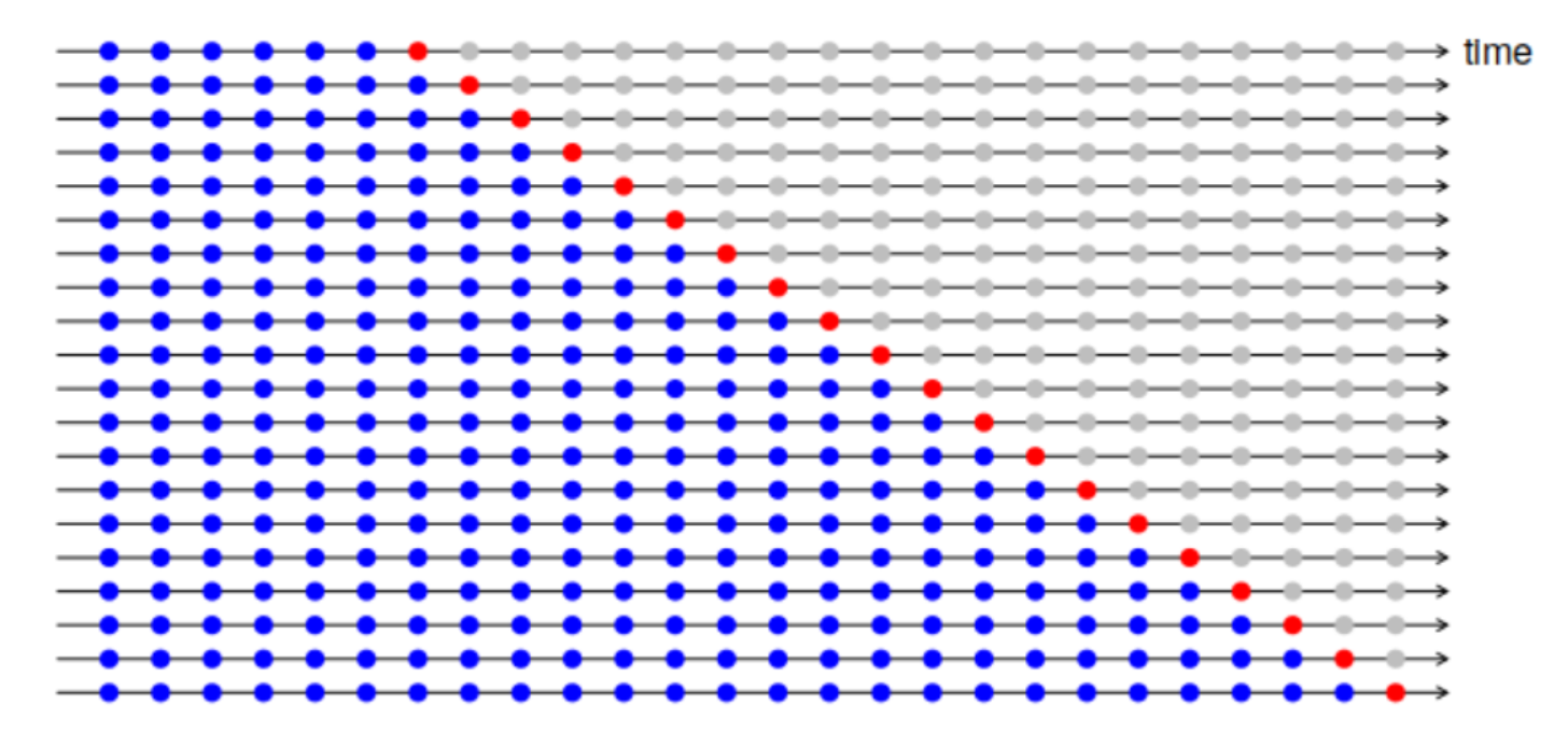
Regarding model accuracy and parameter tuning, we adopt time series split cross validation instead of general cross validation (GCV) to maintain the time series structure and to avoid look-ahead bias. As illustrated below, with blue dots representing training set and orange dots representing cross-validation set, the training window has been expanding through the cross-validation process. After exhausting the whole data set, we calculate the cross validation error (CV error) and choose the hyperparameters that minimize the CV error.

Modeling Schemes

We form a parallel pipeline for our research purposes by proposing three different methods in order to reach a comprehensive conclusion to assess the performances of our models.

Method 1. Simple Split

We first apply a simple training and cross-validation scheme using the first 13 days of our available data as training and cross validation set and the remaining 2 days as test set. \

Method 2: Simple Split with additional previous 5-min features

Method 2 follows a similar rationale to Method 1 except that we believe that modified features from the previous 5 minutes contain information with additional predictive power. \

Method 3: 3-day rolling window with testing set on the remaining 2 days

Due to the nature of time-series analysis, most of the time the model needs to be fitted and trained with the new data before gaining a higher capability of forecasting certain horizons again. Also, it might be true that the structure of data sets change over time and to include the historical data in the “far” past may introduce extra noise. Hence, it makes sense to apply the rolling window approach where we use the previous 3 days to train and cross validate our model and make the prediction in the next day. \

Method 4: 3-day rolling window with testing set on the remaining 2 days

Method 4 modifies Method 3 in resemblance to the first two methods that keep the last 2 days out from the cross-validation procedure to ensure testing %accuracy.

Result Analysis

In this section, we present and compare the model performance results horizontally and vertically. The following tables summarize the Absolute Percentage Error (APE) of models based on various methods.

BAC (%)	Lasso (1 min)	RF (1 min)	Lasso (5 min)	RF (5 min)	Lasso Rolling	RF Rolling	Benchmark
bid-ask spread	0.79	0.79	0.77	0.79	0.81	0.85	0.93
volatility	6.89	12.70	9.49	11.64	7.37	13.39	7.07
minute return	100.00	101.92	100.00	102.92	99.97	103.09	139.57

TSLA (%)	Lasso (1 min)	RF (1 min)	Lasso (5 min)	RF (5 min)	Lasso Rolling	RF Rolling	Benchmark
bid-ask spread	13.82	14.59	12.28	13.96	12.75	12.72	14.02
volatility	7.35	7.53	6.38	7.27	7.32	8.85	7.43
minute return	99.95	102.40	99.94	100.60	100.05	101.62	138.07

GOOG (%)	Lasso (1 min)	RF (1 min)	Lasso (5 min)	RF (5 min)	Lasso Rolling	RF Rolling	Benchmark
bid-ask spread	15.40	16.48	14.28	15.24	19.18	18.71	16.60
volatility	12.37	15.40	10.97	12.66	11.58	26.89	11.57
minute return	99.82	100.92	99.85	100.85	99.43	99.98	142.86

Key Findings

Findings in Model Predictability

1. 5-min training window outperforms 1-min training window

From the analysis, both random forest regressor and LASSO work better in prediction for Google and Tesla when we extend our feature set to include all the features in the previous 5 minutes instead of only the features in the previous 1 minute. This indicates features make impacts on our responses gradually. In fact, from the feature importance score generated by random forest, we find that most of the time, features between the previous 3 minutes and 5 minutes are more often picked and assigned higher weights.

2. Longer training days improve model robustness

We have tried different window lengths to predict our responses and in our experiment, models using 13 days of training window will consistently outperform the models using 3 days window.

Comparison in Different Stocks’ Market Microstructure

1. Minute return is difficult to predict

When examining the features selected by LASSO, we find it picks nothing when we include features in the previous 5 minutes. This indicates that we are essentially using the average value of return to predict. Random Forest does utilize several features, but only to yield worse results than our benchmark. This means it picks only noises. Therefore, we need to find stronger features to predict it.

2. Model improvements are different for different stocks

For example, it is generally hard for our models to outperform benchmark when predicting next-minute volatility for BAC. However, we can decrease the average percent error by almost 1 percent for our best model when predicting volatility for TSLA and GOOG.

3. Same feature has different relationships with responses for different stocks

This is rather a quite interesting finding. When we examine the partial dependence plots to see how predictors interact with responses, we find volatility and minute high-low ratio have different impact on the bid-ask spread. For TSLA and GOOG, when volatility or minute high-low ratio in the previous one or five minutes increase, the bid-ask spread tends to increase. However, bid-ask spread for BAC tends to decrease when volatility or high-low ratio increases.

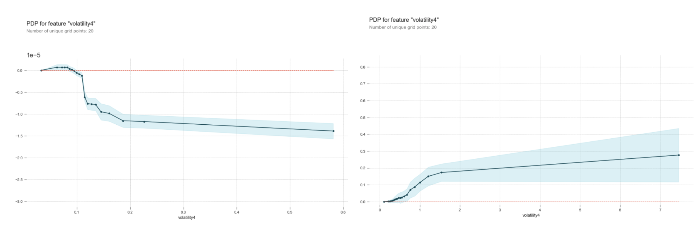
Figure: Partial Dependence Plots for volatility predicting spread, BAC(left) and TSLA

4. Features have different predictability for different stocks

We discover, when predicting bid-ask spread, the top 5 useful features ranked by random forest are the spreads in the previous 5 minutes and perhaps Roll spread for GOOG and TSLA. But for BAC, the top 5 useful features are all estimated volatility in the previous 5 minutes.

Trading Strategy and Market Impact Analysis

From our previous findings, we realize that Lasso with 5-min features input to predict 1-min realized volatility outperforms benchmark on TSLA and GOOG, which has higher predictive power. Based on this finding, we design a trading strategy as follows to trade realized 1-min volatility on those kinds of stocks or index ETFs.

The first trading strategy is to long/short a call or a put and conduct delta hedge if the predicted realized volatility would increase/decrease, which has no delta exposure and positive vega exposure. The intuition is that vega exposure is proportional to the magnitude of implied volatility and it is widely tenable that implied volatility converges to realized volatility.

The second trading strategy is successfully used by some practitioners which is empirical rather than strictly theoretical. This strategy is to long/short straddle and conduct delta hedge if predicted realized volatility is larger/smaller than implied vol. With delta neutral this trading portfolio only has exposures to gamma, vega and theta. Gamma PNL is proportional to realized volatility minus implied volatility. Vega PNL is proportional to implied volatility which could be approximately hedged by VIX if we trade index ETFs. From empirical experience, the Gamma PNL dominates this process hence realized volatility minus implied volatility could be the signal to trade delta-neutral straddle.

Temporary impact is defined as the price change between order initiation and order completion, which has negative effect on order execution. One of the well-known method, Square Root Law of Market Impact, to compare the market impacts among different stocks is the square root law of market impact defined as follows:

\(I(Q)\sim\sigma\left(\frac{\mid Q\mid}{V}\right)^\frac{1}{2}\) where

I(Q) is the expected impact for a traded quantity Q, $\sigma$ is the stock’s daily volatility, $V$ is the average daily volume of the stock and $\frac{Q}{V}$ is the participation rate

Hence in order to screw down the market impact for our trading strategy, we can select the stocks or index ETFs which have relatively low $\sigma V^{-0.5}$. In terms of GOOG and TSLA, we calculate the annualized minute-level volatility divided by square root of average size for every minute and find those of GOOG and TSLA are 21 and 1065 respectively. This means that by trading the same quantity of stocks, the market impact on GOOG is much smaller than that on TSLA. Aiming to ruling out the negative market effect as much as possible, we should trade more on GOOG and less on TSLA based on our trading signals. If the trading strategy is to expanded to a more comprehensive one, a thorough analysis should lead us to a batch of stocks with not only similar microstructure behaviors but also a relatively low square root indicator of market impact.

Conclusion

In this report, we formally present our effort in performing a comparative high-frequency trading analysis on the microstructure behaviors of three common stocks - BAC, GOOG, TSLA - using various feature data inspired by Microstructure in the Machine Age by Easley et al. Using minute as the base unit, we select key features from the paper, including Roll measure, Amihud’s Illiquidity, Volume-synchronized probability of informed trading and estimated volatility, Kyle’s Lambda, and formulate additional features such as high-low ratio, minute return, bid-ask spread and size. Using the features, we mainly apply lasso regression and random forest analysis as machine learning techniques to analyze the next-minute predictability on volatility, spread and return. Through different methods of cross validation, we compare the model performances for all three stocks and realize that a longer training span with variables in longer lookback horizon gives the most promising results in predicting 1-min realized volatility. Based on the model findings, we propose to long/short straddle and vanilla option and conduct delta hedge at that same time to trade predicted volatility signals. To measure the expected market impact of the trade, we propose to allocate different weights to different stocks according to the coefficient of Square Root Law.