Are Solely Price-based Factors Powerful Enough for Cross-sectional Equity Return Predictions: An Empirical Study on the Limited Predictive Power of Momentum-based factors under Machine Learning Framework.

In collaboration with Katherine Liu, Chris Wang and Joe Zhou

This research digs into the predictive powers of price-based variables in US equity stock returns with machine learning tools. We apply multiple classic machine learning models to estimate the probability of the next period return of a stock being above and below the cross-sectional median. The analysis focuses on the predictability of momentum factors with different lookback horizons, which represent the empirically observed tendency for rising asset prices to rise further, and falling prices to keep falling.

The research idea originates from a paper by Borisenko published in 2019: Momentum Investing and Alternative to Deep Learning Methodologies. The original paper discovers findings in price-based variables, especially momentum, in the deep learning realm. However, deep learning models suffer from “black-box” problems such as non-transparency and overfitting. Hence in our project, we are curious about whether more fundamental machine learning models can be applied as an alternative in a similar framework. In addition, we are skeptical about whether we could simply use momentum and market alpha, beta to predict the return. In the case where the result is far from ideal, we want to further analyze the problem and improve the model. Therefore, research is constructed as follows: feature construction, machine learning model building, backtesting strategies and further analysis based on the model performances.

Data and Methodology

Feature Construction

The feature set in the research consists of two categories: momentum factors and market condition variables. The features are subsequently The response will be an indicator of whether the cross-sectional return is above or below the median in the next period.

1. Momentum

Momentum is described as the tendency that winning stocks tend to outperform whereas stocks with falling prices tend to fall even more. In our research project, we construct the momentum variables following the method described in Borisenko’s paper and Lindgren’s paper. We use the following equation to calculate the momentum variable for k = [1,2, …, 21,42, 63, …, 252].

\[MOM_{i,t,K}=\prod_{s=t-2}^{t-K} (1+r_{i,s})-1\]

In the above equation, $r_{i,s}$ denotes the monthly return of stock i on date s where the k subscript denotes the lookback horizon in terms of days. Note that using the above range of k, we are calculating the lookback horizon ranges from one day to one year with the increment being one day for the first month and one month for the rest of the year. Using this method, we generate 32 momentum features, which is the same number as the momentum feature used in Borisenko’s original paper.

2. Market Conditions

The market condition features are generated by the CAPM model:

\[r_{i,\tau}=\hat{\alpha_{i}}+\hat{\beta_{i}}r_{m,\tau}+\epsilon_{i,\tau}\]

where \(\tau \in [t - k, t - 1]\) and \(k = [10, 21. 42, 63, ... , 252]\) days; \(r_{i}\), \(\tau\) is day \(\tau\) return of stock i; \(r_{m,\tau}\) is the market return which we used with the return on the SP 500 index, \(\alpha_{i}\),\(\beta_{i}\) are the stock \(i\)’s loading the on the market risk, pricing error. The procedure for market condition features is constructed through about 5 millions regression coefficients described below.

Market Beta The momentum has a time-varying exposure to the market risk besides the CAPM unconditional relationship between lower beta and lower expected return. After the market climbs, the momentum factor investing in high-beta stocks leads to momentum crashes.

Market Alpha From the FF-3, the alpha could price the cross-section of equity returns and the alpha momentum dominates price momentum in the US. Compared with price momentum, the alpha momentum experiences slower reversions in post-formation periods. Investing in the past alpha delivers less volatile returns compared to investing in price momentum.

Market return and volatility we also use the S&P 500 index to estimate the average market returns and standard deviation of returns over k days ( k = [10, 21, 42, 63, 126, 252]) . There is further analysis reporting the nonlinearity in the relationship between momentum returns and past market performance, which encourages us to apply advanced machine learning models on this problem.

Models and training

Following Borisenko, the prediction is framed as a classification problem to forecast if the cross-sectional return is above or below the median.

\[y_{i,t+1} = \left\{ \begin{array}{ll} 1 & if r_{i,t+1} \geq median(r_{t+1} \\ 0 & otherwise \\ \end{array} \right.\]

For validation, we split the sample into training, validation and testing sets. The training set spans from January 1965 to January 1991 with 137357 observations, the validation from February 1991 to June 2000 with 68516 observations, and the testing from July 2000 to December 2019 with 136571 observations.
To address the classification, we select several machine learning models as alternatives. Candidate models include Logistic Lasso, Linear Discriminant Analysis, Quadratic Discriminant Analysis, Random Forest, XGBoost. For each model, we apply k-fold cross validation algorithms to tune the parameters within the training set; for XGBoost, we perform step-wised hyperparameter tuning to select a set of model parameters to control for the learning process.

1.Walk Forward Analysis

One of the hypotheses why our models might give poor performance is that the processes are not stationary, that the relationship between X and Y changes with time. Therefore, we apply a Walk Forward Analysis (WFA), or rolling window estimation, to prevent the influence of regime shift.

Instead of dividing the data into three sets specified in the previous section, we combined the previous train and validation sets, and formed a new training set for WFA. At time t, we used data from the past three years (36 months) as the training set to train our model, and use data from time t to estimate return at time t+1. Repeat every day, and we can obtain a series of predictions for validation.

2. Portfolio Construction Backtesting

To construct portfolio backtesting for each model, we focus on two datasets. One is the dataset that contains the probability estimate for each ticker on the given date and the other is the monthly return dataset given by WRDS CRSP.

Our backtesting function selects stocks on a monthly basis. For each month, the top 50 stocks with the highest probability as the stocks to long and the bottom 50 stocks with the lowest probability as to construct a short portfolio. Furthermore, the backtesting function is using an equal weight method in building a portfolio with the initial investment cost of 1 dollar.

To calculate the profit for each stock, we use the price of the stock in the next period and subtract it by the price of the stock in the current period. As we use the price of the stock in the next period, an error occurred which caught our attention. Due to the limit of our data and the time frame that we are focusing on, there are cases where the price of the stock in the next period is not available to us. Under this case, we design our function using try and except and manually coded the price of the stock in the next period to be 0.

After calculating the profit generated from each stock and the weight of stock, we generate the profit and loss by subtracting the short positions from the long positions. Repeating this process for each day and calculating the cumulative sum, we obtain a final profit and loss for our strategy generated by each model. \newline

Results and Further Analysis

1. Out-of-Sample Performance

The model predictions are assessed on the validation set. With a base rate of 49.9%, table 1 shows the misclassification rates and the top 1000 scores of the candidate model predictions. The misclassification rate captures the prediction error on the validation set, while the top 1000 score captures the success rate of the top 1000 predicted posterior probability. Figure 1 (left) shows the receiver operating characteristic curves of cross-sectional prediction using the same set of models. Figure 1 (right) shows the ROC result of the robustness check of the data and model performances on the in-period return predictions.

Model	Misclassification Rate	Top 1000 Rate
Logistic Lasso	47.98%	60.40%
Linear Discriminant Analysis	47.89%	65.01%
Quadratic Discriminant Analysis	50.30%	85.97%
Random Forest	48.21%	54.05%
XGBoost	48.93%	52.40%

Table 1. metrics for classification models

With an almost 0% misclassification rate and ideal ROC curves, we can ensure that the constructed features have high explanatory power of in-period returns. However, the models do not generalize well, leaving us very different results from the deep learning framework of the original paper. All misclassification rates are not significantly different from the base rate; regarding the top 1000 rate, tree-based models (random forest and XGBoost) in fact have worse performance than more fundamental ones.

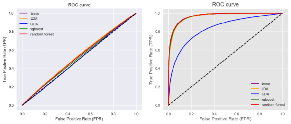
Figure 1: ROC curves for cross-sectional predictions (left) and in-period predictions (right) by each model

Zooming in, we find that the Quadratic Discriminant Analysis achieved a relatively high Top 1000 score despite its mediocre performance on other metrics. Figure 2 shows the predicted posterior probability distribution of the QDA model. The distribution signifies the fact that without an assumption of the class distributions, QDA is able to capture the tail probability relatively well, i.e. allocates higher posterior probabilities on edges and results in the high Top 1000 Sucess rate.

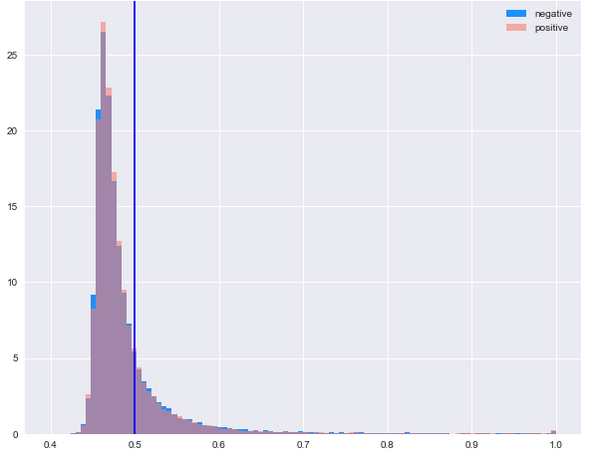
Figure 2. distribution of posterior probabilities by QDA model

2. WFA results

We re-examine the ROC curve, misclassification rate, and top 1000 score after applying WFA on random forest. The improvement is not significantly different from not applying WFA, but the results showed clearer patterns for further analysis.

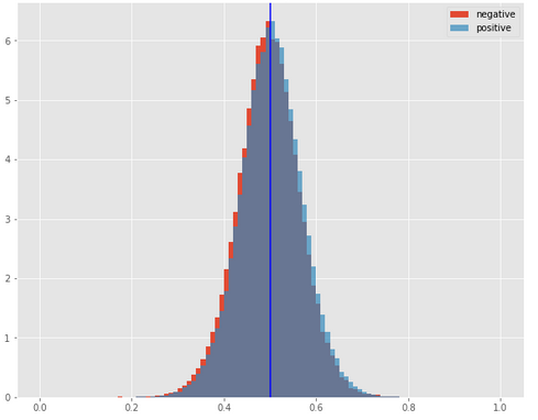
Figure 3. distribution of posterior probabilities by Random Forest model

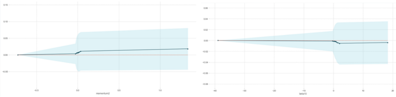
Figure 4. Partial Dependence Plots for features Momentum2 and Beta10

The posterior probability distribution plot showed that the random forest made a separation between two classes. The distribution of class 0’s posterior probability is shifted left.

The partial dependence plots (Figure 4) from random forest also showed some discovery. We picked a representative for each kind of feature, momentum, alpha, beta, and market return. Alpha had no contribution to the distinguishing process. But the classification showed threshold behaviors with respect to momentum, beta, and market return.

We then go back and draw boxplots to identify if there is a relationship between X and Y. Most of the plots showed that some features can provide tiny predictability (full set of graphs in the appendix). For instance, the momentum box plot (Figure 5) indicates a mean reversion effect, i.e. low momentum in the past, high return in the future. Class 1 observations are generally shifted downward compared with class 0 observations, and they were detected by our models.

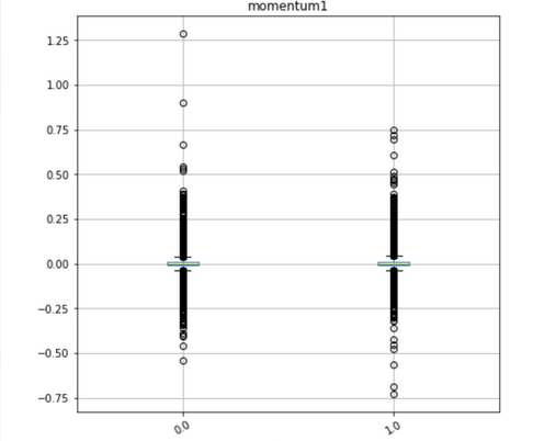
Figure 5. boxplot of feature momentum1 in two response classes

In general, WFA moderately addresses non-stationary issues and provides insights on the model’s performances. Random forest model didn’t fail, it achieved some separation in the data, but the separation is not enough for good classification performance.

3. Backtesting Strategy Performance

Following the backtesting strategy described in section 2.4, we generate a plot of the PnL curve of the combination of long and short strategies for each model. Aside from the curves for the four strategies generated by machine learning models, we also include the PnL curve for S&P 500 index as a benchmark.

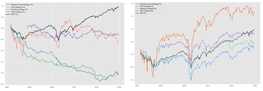
Figure 6. "Long-Short"(left) and "Long-Only"(right) Backtesting PnL Outcome

Examining the plots on the left of Figure 6, we notice that the average performance of the strategies does not outperform our benchmark. In fact, except for the QDA strategy between around 2009 and 2012, none of the strategies in any time period outperform the S&P 500 index. Even though the QDA strategy behaves nicely between 2009 and 2012, topping the benchmark, the performance of the strategy tumbles for the later period. Additionally, we observe that the strategies generated by random forest and XGBoost performed miserably from 2000 to 2016. Even though the performance of both strategies improves from 2016, the improvement is not enough to compensate for the loss in the previous time period.

Instead of using the long-short strategy proposed by the paper, we decide to adopt a long-only strategy based on our machine learning models. The long-only strategy selects the top 50 stocks with the highest estimated probability and constructs a portfolio using equal weight. Now, we observe that the PnL generated by the QDA model and the walk forward outperforms the benchmark PnL. As we are selecting the top 50 stocks, the long-only strategy leverages the comparative advantage of the QDA model with a high top 1000 rate, causing the portfolio to outperform the benchmark.

Aside from the curve, we also calculate the Sharpe ratio for both long-short and long-only strategies generated by the 4 models, which is shown in table x and x. For the long-short strategy, the highest Sharpe ratio is achieved by QDA strategy which is in-line with our analysis above. For the long-only strategy, the QDA strategy achieves a Sharpe ratio of over 1, which indicates that the strategy is good. This also accords with the above analysis as well.

Model	Long Short Strategy Sharpe Ratio	Long Only Strategy Sharpe Ratio
Quadratic Discriminant Analysis	0.3954	1.0283
Random Forest	0.0684	0.3528
XGBoost	0.1263	0.4167
Walk Forward Analysis	0.0765	0.9918

Table 2. Sharpe Ratios of backtesting strategies

Conclusion

We research on the predictability of price-based variables, especially momentum factors and market conditions, in the machine learning framework. With the findings that most of the candidate models do not generalize well through data validation and backtesting, we conclude that momentum and market condition factors by themselves are not sufficient to generate reliable predictions on relative stock returns.
Walk forward analysis on the random forest model moderately addresses the non-stationarity problem in time-series data, i.e. change of regimes in different time frames. However, the rolling windows of train-test analysis do not significantly improve the model metrics.

Our machine learning models, especially the Quadratic Discriminative Analysis, is capable of capturing the tail distribution in the posterior probability prediction, which results in a high top success rate. Incorporating this finding, we propose an alternative backtesting strategy from the original paper. The PnL and Sharpe Ratios of the modified strategy show an improvement in the backtesting momentum portfolio generated by machine learning models and some portfolios significantly outperformed the benchmark portfolio.

As a conclusion, the Borisenko paper’s deep learning methodology is not replicable in a more general and fundamental machine learning framework. Though specific trading strategies can be derived from modeling findings, most machine learning models are not capable of generating solid classifications with pure price-based variables.